Sports Franchise Values

A 9Ware Workshop Regression Analysis Project

Do attendance and/or social media follower counts explain the huge variation in franchise values across Major League Baseball and the National Football League? We thought we'd find out.

Given our continuing fascination with data related to sports, business, and sports business, we decided to do some regression analysis to see if fanbase counts can predict franchise values in the MLB and NFL. And if so, we wanted to know what part of the fanbase does a better job of it -- attendance or social media followers. We gathered the data from various sources^* and started with a visual assessment -- scatterplots with linear regression lines and their 95% confidence intervals (shaded)....

MLB

NFL

[Franchise values in $millions]

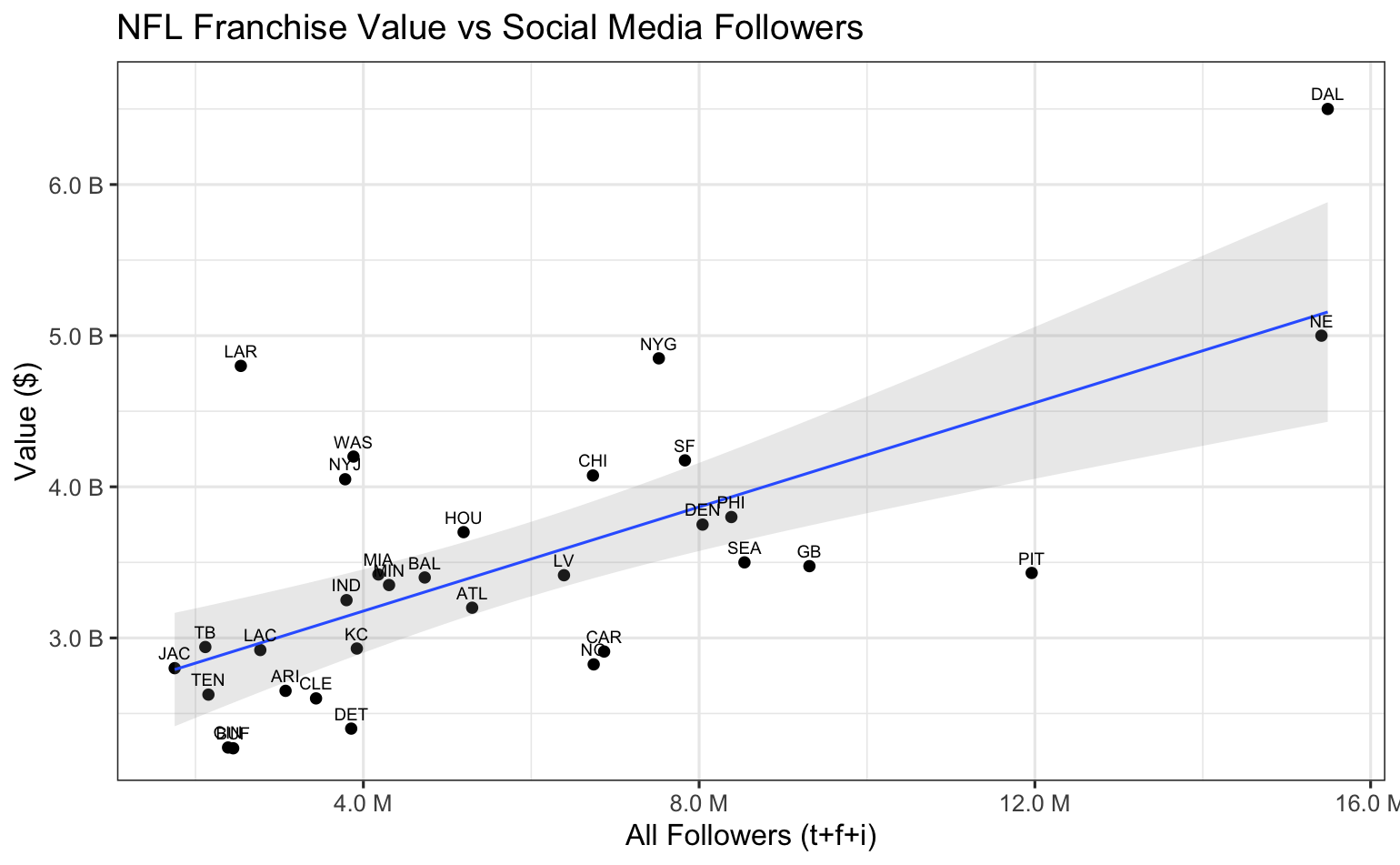
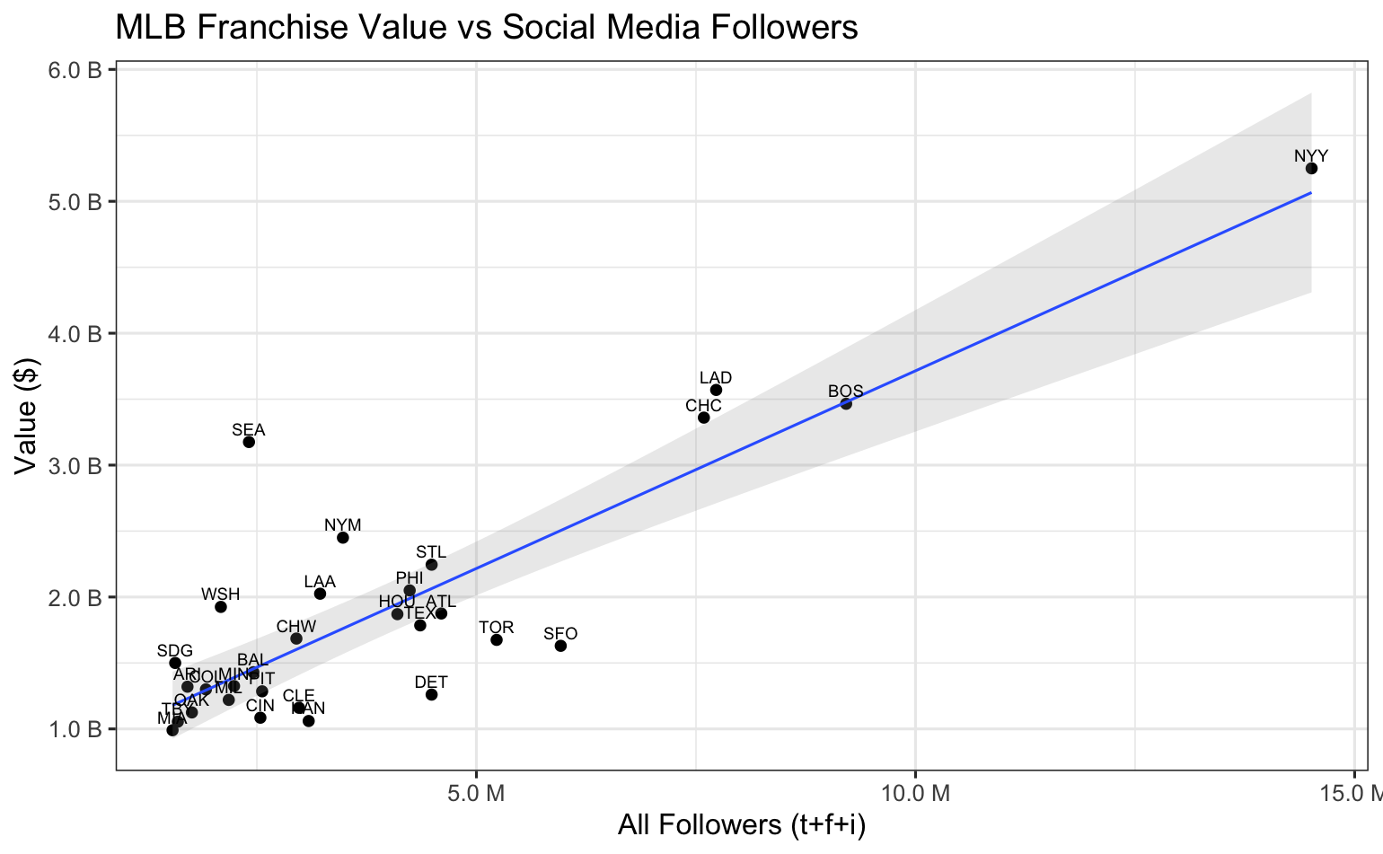
We see some useful observations here. First, MLB attendance appears to be a good indicator of franchise value. However, most of the NFL teams are clustered in a nearly circular pattern showing little linear connection with franchise value. This is not too surprising because media rights are such a huge part of the NFL revenue model, especially compared to game day revenue across only eight home games.

Now let's compare the social media follower charts. The MLB chart is difficult to decipher as shown here because the 15 million(!) Yankees followers have caused most of the other teams to bunch up in the lower left corner, but even the 'bunching' appears more random than linear. On the other hand, the NFL followers chart does show promise for a meaningful linear relationship to franchise values.

Ok, let's get into some regression analysis. For each league we ran three regressions (value ~ attendance), (value ~ followers), and (value ~ attendance & followers). Here are the results:

MLB Regression Results

Brief |
Full

----------
Regression: data$value ~ data$attendance
Residual standard error: 744.6 on 28 degrees of freedom
Multiple R-squared:  0.4371,	Adjusted R-squared:  0.417
F-statistic: 21.74 on 1 and 28 DF,  p-value: 6.968e-05

----------
Regression: data$value ~ data$all_followers)
Residual standard error: 509.8 on 28 degrees of freedom
Multiple R-squared:  0.7362,	Adjusted R-squared:  0.7268
F-statistic: 78.14 on 1 and 28 DF,  p-value: 1.361e-09

----------
Regression: data$value ~ data$attendance + data$all_followers
Residual standard error: 509.8 on 28 degrees of freedom
Multiple R-squared:  0.8111,	Adjusted R-squared:  0.7971
F-statistic: 57.96 on 2 and 27 DF,  p-value: 1.698e-10

--------------------
AIC Model Comparison:
              K   AICc Delta_AICc AICcWt Cum.Wt      LL
att+fol       4 456.69       0.00   0.98   0.98 -223.54
followers     3 464.03       7.34   0.02   1.00 -228.55
attendance    3 486.76      30.08   0.00   1.00 -239.92

----------

Call:
lm(formula = data$value ~ data$attendance)

Residuals:
     Min       1Q   Median       3Q      Max
-1182.13  -444.26   -41.18   251.85  2554.89

Coefficients:
                 Estimate Std. Error t value Pr(>|t|)
(Intercept)     -42.72074  439.26954  -0.097    0.923
data$attendance   0.08293    0.01779   4.663 6.97e-05 ***
---
Signif. codes:  0 ‘***’ 0.001 ‘**’ 0.01 ‘*’ 0.05 ‘.’ 0.1 ‘ ’ 1

Residual standard error: 744.6 on 28 degrees of freedom
Multiple R-squared:  0.4371,	Adjusted R-squared:  0.417
F-statistic: 21.74 on 1 and 28 DF,  p-value: 6.968e-05

----------

Call:
lm(formula = data$value ~ data$all_followers)

Residuals:
    Min      1Q  Median      3Q     Max
-874.29 -216.36  -44.89  182.82 1734.62

Coefficients:
                    Estimate Std. Error t value Pr(>|t|)
(Intercept)        7.181e+02  1.634e+02   4.396 0.000144 ***
data$all_followers 2.997e-04  3.390e-05   8.840 1.36e-09 ***
---
Signif. codes:  0 ‘***’ 0.001 ‘**’ 0.01 ‘*’ 0.05 ‘.’ 0.1 ‘ ’ 1

Residual standard error: 509.8 on 28 degrees of freedom
Multiple R-squared:  0.7362,	Adjusted R-squared:  0.7268
F-statistic: 78.14 on 1 and 28 DF,  p-value: 1.361e-09

----------

Call:
lm(formula = data$value ~ data$attendance + data$all_followers)

Residuals:
    Min      1Q  Median      3Q     Max
-571.91 -338.04    3.01  170.80 1508.72

Coefficients:
                    Estimate Std. Error t value Pr(>|t|)
(Intercept)        6.027e+00  2.592e+02   0.023  0.98162
data$attendance    3.946e-02  1.206e-02   3.271  0.00293 **
data$all_followers 2.455e-04  3.358e-05   7.311 7.29e-08 ***
---
Signif. codes:  0 ‘***’ 0.001 ‘**’ 0.01 ‘*’ 0.05 ‘.’ 0.1 ‘ ’ 1

Residual standard error: 439.3 on 27 degrees of freedom
Multiple R-squared:  0.8111,	Adjusted R-squared:  0.7971
F-statistic: 57.96 on 2 and 27 DF,  p-value: 1.698e-10

sma
744.6172  - Residual Standard Error
15524733  - Sum Squared Error
517491.1  - Mean Squared Error
0.4371058  - Multiple R-squared
0.4170025 - Adjusted R-squared

sms
509.7522  - Residual Standard Error
7275725  - Sum Squared Error
242524.2  - Mean Squared Error
0.7361975  - Multiple R-squared
0.726776 - Adjusted R-squared

smas
439.2982  - Residual Standard Error
5210538  - Sum Squared Error
173684.6  - Mean Squared Error
0.8110768  - Multiple R-squared
0.7970825 - Adjusted R-squared

Model selection based on AICc:
              K   AICc Delta_AICc AICcWt Cum.Wt      LL
att+fol       4 456.69       0.00   0.98   0.98 -223.54
followers     3 464.03       7.34   0.02   1.00 -228.55
attendance    3 486.76      30.08   0.00   1.00 -239.92

NFL Regression Results

Brief |
Full

----------
Regression: data$value ~ data$attendance
Residual standard error: 752.3 on 30 degrees of freedom
Multiple R-squared:  0.3347,	Adjusted R-squared:  0.3125
F-statistic: 15.09 on 1 and 30 DF,  p-value: 0.0005236

----------
Regression: data$value ~ data$all_followers
Residual standard error: 681.4 on 30 degrees of freedom
Multiple R-squared:  0.4543,	Adjusted R-squared:  0.4361
F-statistic: 24.97 on 1 and 30 DF,  p-value: 2.349e-05

----------
Regression: data$value ~ data$attendance + data$all_followers
Residual standard error: 640.4 on 29 degrees of freedom
Multiple R-squared:  0.5339,	Adjusted R-squared:  0.5018
F-statistic: 16.61 on 2 and 29 DF,  p-value: 1.557e-05

--------------------
AIC Model Comparison:
              K   AICc Delta_AICc AICcWt Cum.Wt      LL
att+fol       4 510.72       0.00   0.76   0.76 -250.62
followers     3 513.15       2.43   0.23   0.99 -253.14
attendance    3 519.49       8.77   0.01   1.00 -256.31

----------

Call:
lm(formula = data$value ~ data$attendance)

Residuals:
     Min       1Q   Median       3Q      Max
-1307.85  -473.77   -54.69   497.78  1585.54

Coefficients:
                  Estimate Std. Error t value Pr(>|t|)
(Intercept)     -866.26473 1127.68150  -0.768 0.448384
data$attendance    0.06504    0.01674   3.885 0.000524 ***
---
Signif. codes:  0 ‘***’ 0.001 ‘**’ 0.01 ‘*’ 0.05 ‘.’ 0.1 ‘ ’ 1

Residual standard error: 752.3 on 30 degrees of freedom
Multiple R-squared:  0.3347,	Adjusted R-squared:  0.3125
F-statistic: 15.09 on 1 and 30 DF,  p-value: 0.0005236

----------

Call:
lm(formula = data$value ~ data$all_followers)

Residuals:
    Min      1Q  Median      3Q     Max
-1119.2  -465.1  -128.4   237.6  1873.6

Coefficients:
                    Estimate Std. Error t value Pr(>|t|)
(Intercept)        2.489e+03  2.327e+02  10.695 9.35e-12 ***
data$all_followers 1.722e-04  3.447e-05   4.997 2.35e-05 ***
---
Signif. codes:  0 ‘***’ 0.001 ‘**’ 0.01 ‘*’ 0.05 ‘.’ 0.1 ‘ ’ 1

Residual standard error: 681.4 on 30 degrees of freedom
Multiple R-squared:  0.4543,	Adjusted R-squared:  0.4361
F-statistic: 24.97 on 1 and 30 DF,  p-value: 2.349e-05

----------

Call:
lm(formula = data$value ~ data$attendance + data$all_followers)

Residuals:
    Min      1Q  Median      3Q     Max
-906.17 -422.11  -20.93  308.58 1575.46

Coefficients:
                    Estimate Std. Error t value Pr(>|t|)
(Intercept)        2.841e+02  1.014e+03   0.280  0.78132
data$attendance    3.651e-02  1.640e-02   2.227  0.03389 *
data$all_followers 1.312e-04  3.727e-05   3.521  0.00144 **
---
Signif. codes:  0 ‘***’ 0.001 ‘**’ 0.01 ‘*’ 0.05 ‘.’ 0.1 ‘ ’ 1

Residual standard error: 640.4 on 29 degrees of freedom
Multiple R-squared:  0.5339,	Adjusted R-squared:  0.5018
F-statistic: 16.61 on 2 and 29 DF,  p-value: 1.557e-05

sma
752.3046  - Residual Standard Error
16978867  - Sum Squared Error
530589.6  - Mean Squared Error
0.334681  - Multiple R-squared
0.3125037 - Adjusted R-squared

sms
681.3525  - Residual Standard Error
13927236  - Sum Squared Error
435226.1  - Mean Squared Error
0.4542595  - Multiple R-squared
0.4360682 - Adjusted R-squared

smas
640.4129  - Residual Standard Error
11893731  - Sum Squared Error
371679.1  - Mean Squared Error
0.5339426  - Multiple R-squared
0.5018008 - Adjusted R-squared

Model selection based on AICc:
              K   AICc Delta_AICc AICcWt Cum.Wt      LL
att+fol       4 510.72       0.00   0.76   0.76 -250.62
followers     3 513.15       2.43   0.23   0.99 -253.14
attendance    3 519.49       8.77   0.01   1.00 -256.31

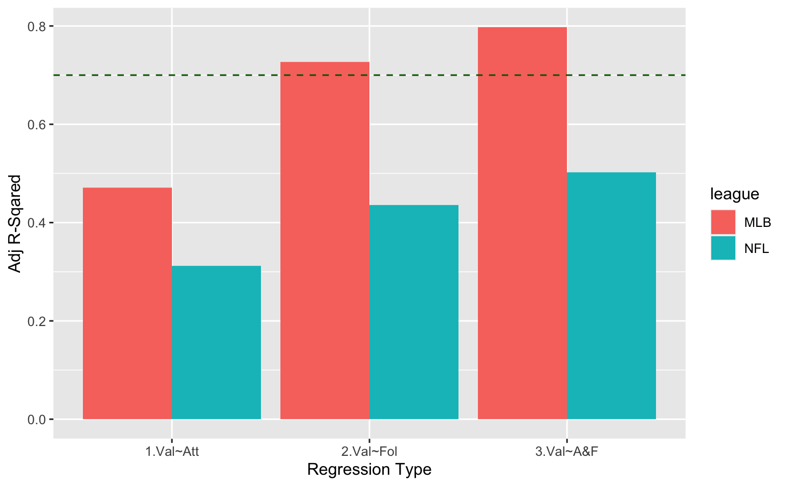
There are many ways to assess and compare different linear regression models. One of the clearest metrics for our purposes here is the R-Squared value, a number indicating the proportion of the variation in the dependent variable (franchise value) that is described by the predictor variables (attendance, followers, or attendance&followers). Actually, we'll focus on the Adjusted R-Squared value, which adjusts R-Squared for the number of predictor variables used. Adjusted R-Squared is always less than or equal to R-Squared, decreasing with the addition of more variables that don't contribute much to the overall analysis.

Adjusted R-Squared Comparisons

Regression	MLB	NFL
Value~Attendance	0.4170	0.3125
Value~Followers	0.7268	0.4361
Value~Att&Fol	0.7971	0.5018

The green dashed line above represents the point where 70% of the variation in franchise value is explained by the model. And for MLB teams, followers alone as well as the combination of attendance and followers get us there (0.7268, 0.7971). This means that most of the regression fit comes from followers, but adding the weaker attendance variable meaningfully adds to the predictability of the model. We confirmed that with an Akaike information criterion (AIC) model comparison at the bottom of the output above. The AIC metric finds the model that explains the most variation in the data, while penalizing models that use an excessive number of parameters. [Read more about AIC here.]

So, we're satisfied with our results on the MLB side of things -- that attendance and follower counts work together to sufficiently describe variations in franchise values (to the 70% benchmark we chose to target).

We have a different situation on the NFL side, as our maximum Adjusted R-Squared value here indicates that we are barely explaining 50% of franchise values, even with the combination of attendance and follower counts. Taking another look at the initial visualizations, we noticed that the teams below the regression lines in both charts are generally in small markets, while the teams above the lines are generally in large markets. So we obtained metro area population data for NFL teams from www.census.gov to see if adding this as a third NFL predictor variable might improve things. Starting with a scatterplot of franchise values vs metro area populations...

Metro area population sizes alone don't look too promising as a predictor variable, but adding it to the regression analysis could tell a different story given the clear separation of small vs large population sizes shown in the earlier scatterplots.

NFL Regression Results with Metro Populations Added

Brief |
Full

----------
Regression: data$value ~ data$population
Residual standard error: 796.1 on 30 degrees of freedom
Multiple R-squared:  0.2549,	Adjusted R-squared:  0.2301
F-statistic: 10.26 on 1 and 30 DF,  p-value: 0.003208

----------
Regression: data$value ~ data$attendance + data$population
Residual standard error: 654.4 on 29 degrees of freedom
Multiple R-squared:  0.5134,	Adjusted R-squared:  0.4798
F-statistic:  15.3 on 2 and 29 DF,  p-value: 2.913e-05

----------
Regression: data$value ~ data$all_followers + data$population
Residual standard error: 504 on 29 degrees of freedom
Multiple R-squared:  0.7113,	Adjusted R-squared:  0.6914
F-statistic: 35.73 on 2 and 29 DF,  p-value: 1.499e-08

----------
Regression: data$value ~ data$attendance + data$all_followers data$population
Residual standard error: 477.3 on 28 degrees of freedom
Multiple R-squared:   0.75,	Adjusted R-squared:  0.7232
F-statistic:    28 on 3 and 28 DF,  p-value: 1.412e-08

--------------------
AIC Model Comparison:
            K   AICc Delta_AICc AICcWt Cum.Wt      LL
att+fol+pop 5 493.61       0.00   0.71   0.71 -240.65
fol+pop     4 495.39       1.78   0.29   1.00 -242.95
att+fol     4 510.72      17.11   0.00   1.00 -250.62
att+pop     4 512.10      18.49   0.00   1.00 -251.31
followers   3 513.15      19.53   0.00   1.00 -253.14
attendance  3 519.49      25.87   0.00   1.00 -256.31
population  3 523.11      29.50   0.00   1.00 -258.13

----------

Call:
lm(formula = data$value ~ data$population)

Residuals:
     Min       1Q   Median       3Q      Max
-1296.16  -387.92    21.43   233.74  2815.99

Coefficients:
                 Estimate Std. Error t value Pr(>|t|)
(Intercept)     2.986e+03  2.096e+02  14.250 6.79e-15 ***
data$population 9.252e-05  2.888e-05   3.204  0.00321 **
---
Signif. codes:  0 ‘***’ 0.001 ‘**’ 0.01 ‘*’ 0.05 ‘.’ 0.1 ‘ ’ 1

Residual standard error: 796.1 on 30 degrees of freedom
Multiple R-squared:  0.2549,	Adjusted R-squared:  0.2301
F-statistic: 10.26 on 1 and 30 DF,  p-value: 0.003208

----------

Call:
lm(formula = data$value ~ data$attendance + data$population)

Residuals:
     Min       1Q   Median       3Q      Max 
-1053.09  -466.26   -73.81   349.40  1617.12 

Coefficients:
                  Estimate Std. Error t value Pr(>|t|)    
(Intercept)     -8.042e+02  9.811e+02  -0.820 0.419064    
data$attendance  5.781e-02  1.473e-02   3.925 0.000491 ***
data$population  7.835e-05  2.401e-05   3.263 0.002821 ** 
---
Signif. codes:  0 ‘***’ 0.001 ‘**’ 0.01 ‘*’ 0.05 ‘.’ 0.1 ‘ ’ 1

Residual standard error: 654.4 on 29 degrees of freedom
Multiple R-squared:  0.5134,	Adjusted R-squared:  0.4798 
F-statistic:  15.3 on 2 and 29 DF,  p-value: 2.913e-05

----------

Call:
lm(formula = data$value ~ data$all_followers + data$population)

Residuals:
   Min     1Q Median     3Q    Max
-838.2 -321.0  -29.2  285.7 1139.6

Coefficients:
                    Estimate Std. Error t value Pr(>|t|)
(Intercept)        1.987e+03  1.985e+02  10.012 6.43e-11 ***
data$all_followers 1.726e-04  2.550e-05   6.771 1.97e-07 ***
data$population    9.291e-05  1.828e-05   5.082 2.02e-05 ***
---
Signif. codes:  0 ‘***’ 0.001 ‘**’ 0.01 ‘*’ 0.05 ‘.’ 0.1 ‘ ’ 1

Residual standard error: 504 on 29 degrees of freedom
Multiple R-squared:  0.7113,	Adjusted R-squared:  0.6914
F-statistic: 35.73 on 2 and 29 DF,  p-value: 1.499e-08

----------

Call:
lm(formula = data$value ~ data$attendance + data$all_followers +
    data$population)

Residuals:
    Min      1Q  Median      3Q     Max
-623.22 -344.98  -96.32  270.66 1113.25

Coefficients:
                    Estimate Std. Error t value Pr(>|t|)
(Intercept)        4.610e+02  7.566e+02   0.609   0.5472
data$attendance    2.584e-02  1.241e-02   2.082   0.0466 *
data$all_followers 1.436e-04  2.789e-05   5.148 1.85e-05 ***
data$population    8.651e-05  1.759e-05   4.920 3.45e-05 ***
---
Signif. codes:  0 ‘***’ 0.001 ‘**’ 0.01 ‘*’ 0.05 ‘.’ 0.1 ‘ ’ 1

Residual standard error: 477.3 on 28 degrees of freedom
Multiple R-squared:   0.75,	Adjusted R-squared:  0.7232
F-statistic:    28 on 3 and 28 DF,  p-value: 1.412e-08


mp
796.1272  - Residual Standard Error
19014554  - Sum Squared Error
594204.8  - Mean Squared Error
0.2549123  - Multiple R-squared
0.230076 - Adjusted R-squared

msp
504.017  - Residual Standard Error
7366961  - Sum Squared Error
230217.5  - Mean Squared Error
0.7113247  - Multiple R-squared
0.6914161 - Adjusted R-squared

map
654.3906  - Residual Standard Error
12418583  - Sum Squared Error
388080.7  - Mean Squared Error
0.5133763  - Multiple R-squared
0.479816 - Adjusted R-squared

masp
477.3202  - Residual Standard Error
6379368  - Sum Squared Error
199355.3  - Mean Squared Error
0.7500236  - Multiple R-squared
0.7232405 - Adjusted R-squared

Model selection based on AICc:
            K   AICc Delta_AICc AICcWt Cum.Wt      LL
att+fol+pop 5 493.61       0.00   0.71   0.71 -240.65
fol+pop     4 495.39       1.78   0.29   1.00 -242.95
att+fol     4 510.72      17.11   0.00   1.00 -250.62
att+pop     4 512.10      18.49   0.00   1.00 -251.31
followers   3 513.15      19.53   0.00   1.00 -253.14
attendance  3 519.49      25.87   0.00   1.00 -256.31
population  3 523.11      29.50   0.00   1.00 -258.13

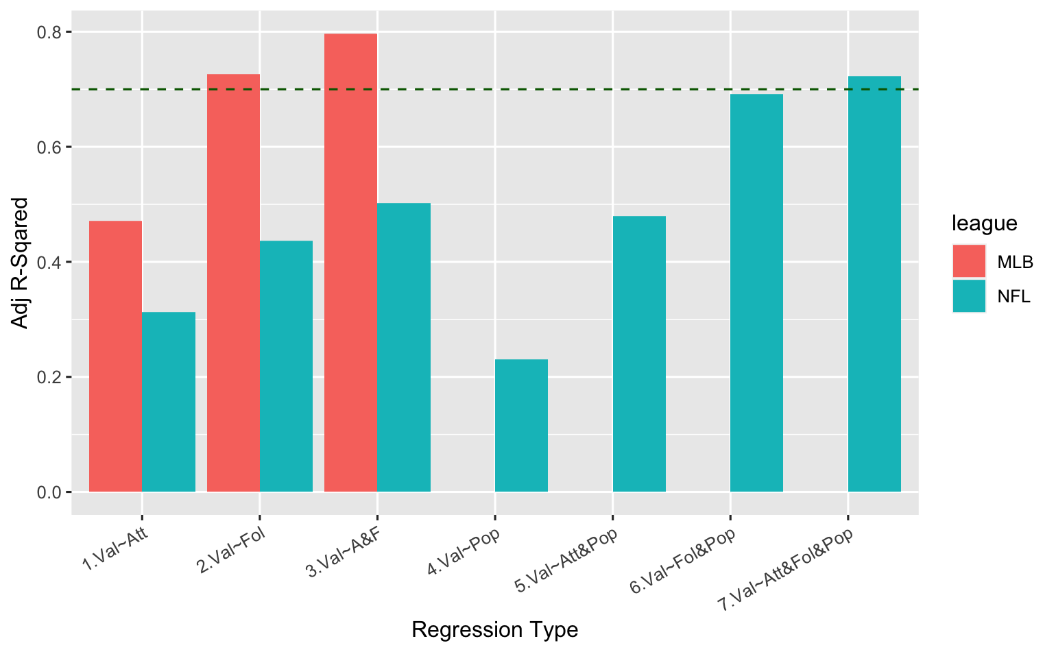
Here are the Adjusted R-Squared values again, including the three new NFL models that consider metro area populations...

Adjusted R-Squared Comparisons

Regression	MLB	NFL
Value~Attendance	0.4170	0.3125
Value~Followers	0.7268	0.4361
Value~Att&Fol	0.7971	0.5018
Value~Pop		0.2301
Value~Att&Pop		0.4798
Value~Fol&Pop		0.6914
Value~Att&Fol&Pop		0.7232

It's not surprising to see here that metro area population alone is indeed a lousy metric -- in fact, it turns out to be the worst predictor of all, explaining a mere 23% of the variance in NFL franchise values! However, it has clearly contributed to the predictive capability of the other NFL variables, significantly improving all of the prior models when added to them. The NFL model that combines attendance, followers and population has the highest Adjusted R-Squared value, and also proves to be the best based on AIC model analysis, as shown at the bottom of the data output above.

Thus, by adding metro area populations to the NFL model, we have surpassed our target of explaining at least 70% of the variation in MLB and NFL franchise values based on average attendance and social media follower counts. Here are the two models we've chosen to best explain the variance in MLB and NFL franchise values, respectively:

Chosen MLB Regression

79%+ of franchise values explained by the model

----------
Regression: data$value ~ data$attendance + data$all_followers
                    Estimate Std. Error t value Pr(>|t|)
(Intercept)        6.027e+00  2.592e+02   0.023  0.98162
data$attendance    3.946e-02  1.206e-02   3.271  0.00293 **
data$all_followers 2.455e-04  3.358e-05   7.311 7.29e-08 ***

---
Residual standard error: 439.3 on 27 degrees of freedom
Multiple R-squared:  0.8111,	Adjusted R-squared:  0.7971
F-statistic: 57.96 on 2 and 27 DF,  p-value: 1.698e-10

--------------------
AIC Model Comparison:
              K   AICc Delta_AICc AICcWt Cum.Wt      LL
att+fol       4 456.69       0.00   0.98   0.98 -223.54
followers     3 464.03       7.34   0.02   1.00 -228.55
attendance    3 486.76      30.08   0.00   1.00 -239.92

Chosen NFL Regression

72%+ of franchise values explained by the model

----------
Regression: data$value ~ data$attendance + data$all_followers + data$population
                    Estimate Std. Error t value Pr(>|t|)
(Intercept)        4.610e+02  7.566e+02   0.609   0.5472
data$attendance    2.584e-02  1.241e-02   2.082   0.0466 *
data$all_followers 1.436e-04  2.789e-05   5.148 1.85e-05 ***
data$population    8.651e-05  1.759e-05   4.920 3.45e-05 ***
---
Residual standard error: 477.3 on 28 degrees of freedom
Multiple R-squared:   0.75,	Adjusted R-squared:  0.7232
F-statistic:    28 on 3 and 28 DF,  p-value: 1.412e-08

--------------------
AIC Model Comparison:
            K   AICc Delta_AICc AICcWt Cum.Wt      LL
att+fol+pop 5 493.61       0.00   0.71   0.71 -240.65
fol+pop     4 495.39       1.78   0.29   1.00 -242.95
att+fol     4 510.72      17.11   0.00   1.00 -250.62
att+pop     4 512.10      18.49   0.00   1.00 -251.31
followers   3 513.15      19.53   0.00   1.00 -253.14
attendance  3 519.49      25.87   0.00   1.00 -256.31
population  3 523.11      29.50   0.00   1.00 -258.13

While we could obviously continue the regression process by gathering more data and trying out additional predictor variables to get to a more respectable Adjusted R-Squared level (say, beyond 90%), we'll stop here and examine the current results...

Interpreting The Results

MLB

For the MLB, the coefficients of 3.946e-02 (attendance) and 2.455e-04 (followers) mean that, on average, franchise value rises $1M for every

(1/3.946e-02) = 25.3 increase in average attendance, and
(1/2.455e-04) = 4,073 increase in social media followers

NFL

For the NFL, the coefficients of 2.584e-02 (attendance), 1.436e-04 (followers) and 8.651e-05 (population) mean that, on average, franchise value rises $1M for every

(1/2.584e-02) = 38.7 increase in average attendance,
(1/1.436e-04) = 6,964 increase in social media followers, and
(1/8.651e-05) = 11,559 increase in metro area population

These relationships as stated explain 70-80% of differences in franchise values. If we were to continue the analysis, we would test some more factors such as number of titles won, number of times reaching the playoffs, years of existence, and of course MLB metro area population sizes... in order to continue improving the model and explain more of the franchise value variations while taking care to not overfit the data.

Wrap Up

This exercise is an example of linear regression analysis. We started with a logical premise -- in our case that attendance and social media follower counts should have some level of impact on franchise value variations, hopefully explaining at least 70% of these variations across teams. We first took a visual look at correlations on scatterplots, then we ran some regressions, reviewed the results, and re-inspected the scatterplots to see whether we had missed something relevant -- in our case that metro area populations might improve the model. Then we ran new regressions based on this re-inspection, reached reasonable 'final' models, and interpreted those results.

Perhaps most importantly, we didn't overfit the data or overthink the results. In most real-world cases, including this one, countless factors are involved in determining something like the value of a franchise, business, product, service, etc. Regression analysis can provide an important and useful partial perspective on the overall situation for your business.

If you made it this far, well, you must really like statistics. Thanks for reading!

^*We used MLB and NFL attendance figures from ESPN, averaging per-game attendance across 2019 and 2021 due to the pandemic. For social media follower counts, we used statista.com. And finally, Forbes provided our franchise values.